Benchmarking Data

Author

Jori Kandra

This training was originally presented as a workshop at EARNCon 2023.

Publication: Older workers were devastated by the pandemic downturn and continue to face adverse employment outcomes

import packages

# import packages
library(tidyverse)
library(epiextractr)
library(here)

Define CPS years

cps_years <- 2007:2020

cps_vars <- c("year", "month", "age", "female", "emp", "basicwgt")

# import basic CPS data
cps_data <- load_basic(cps_years, all_of(cps_vars)) %>% 
  # restrict to 16+
  filter(age >= 16) %>% 
  # create age categories
  mutate(age_group = case_when(
    age <= 24 ~ "16–24 years old",
    age >= 25 & age <= 54 ~ "25–54 years old",
    age >= 55 & age <= 64 ~ "55–64 years old",
    age >= 65 ~ "65+ years old"),
    # adjust weight
    wgt = basicwgt/12)

Using EPI CPS Basic Monthly Extracts, Version 1.0.59

https://www.bls.gov/cps/aa2020/cpsaat18b.htm

cps_data %>% 
  # restrict to employed
  filter(emp == 1, year == 2020) %>% 
  # weighted employment count by year
  group_by(year) %>% tally(wt = wgt) %>% mutate(n = n/1000)

# A tibble: 1 × 2
   year       n
  <int>   <dbl>
1  2020 147795.

# age category benchmark: https://www.bls.gov/cps/aa2020/cpsaat03.htm
cps_data %>% 
  # restrict to employed
  filter(emp == 1, year == 2020) %>% 
  # weighted employment count by year
  group_by(year, age_group) %>% tally(wt = wgt) %>% mutate(n = n/1000) %>% 
  # reshape data
  pivot_wider(id_cols = year, names_from = age_group, values_from = n)

# A tibble: 1 × 5
# Groups:   year [1]
   year `16–24 years old` `25–54 years old` `55–64 years old` `65+ years old`
  <int>             <dbl>             <dbl>             <dbl>           <dbl>
1  2020            17192.            95310.            25469.           9824.

Figure C: change in employment-to-population ratio across age categories

emp <- cps_data %>%
  # isolate recession beginning and end years
  filter(!is.na(emp),
      year %in% c(2007, 2011, 2019, 2020)) %>% 
  # weighted employment * population count by year and age group
  group_by(year, age_group) %>% summarise(emp = sum(emp * wgt), pop = sum(wgt)) %>% 
  # calculate EPOPs
  mutate(epop = emp/pop) %>% pivot_wider(id_cols = age_group, names_from = year, values_from = epop) %>% 
  # calculate percent change in EPOPs
  transmute(age_group = age_group, `2007–2011` = `2011`-`2007`, `2019–2020` = `2020`-`2019`) %>%
  # output to output folder
  write_csv(here("output/older_worker_epop.csv"))

`summarise()` has grouped output by 'year'. You can override using the
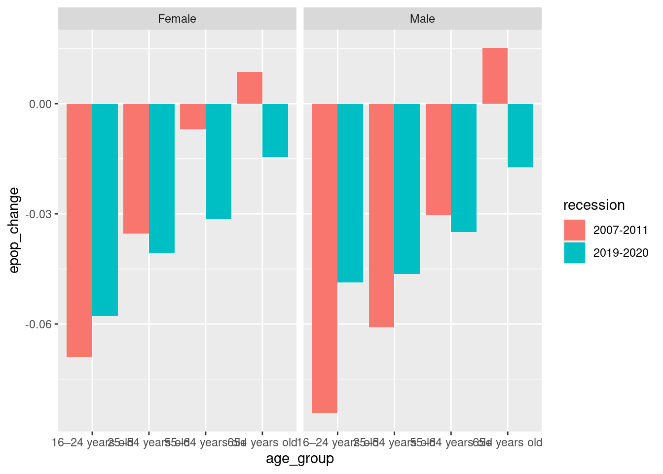
`.groups` argument.

Figure D: Change in employment-population ratios during the Great Recession and the COVID-19 recession, 2007–2011 and 2019–2020, by gender and older age group

epop_gender <- cps_data %>% 
  # isolate recession beginning and end years
  filter(!is.na(emp),
      year %in% c(2007, 2011, 2019, 2020)) %>% 
  # assign value of female as character label ("Female" instead of 1 and "Male" instead of 0)
  #note: requires the installation of haven
  #note: using double ":" is a way of referencing functions in a package without importing entire package
  mutate(female = as.character(haven::as_factor(female))) %>% 
  # weighted employment * population count by year and age group AND female
  group_by(year, age_group, female) %>% summarise(emp = sum(emp * wgt), pop = sum(wgt)) %>% 
  # calculate epops
  mutate(epop = emp/pop) %>% ungroup() %>% 
  # reshape wider to calculate change in EPOPs over recession time perios
  pivot_wider(id_cols = c("age_group", "female"), names_from = year, values_from = epop) %>% 
  # calculate percent change in EPOPs
  transmute(age_group = age_group, female = female, 
            `2007-2011` = `2011` - `2007`, `2019-2020` = `2020` - `2019`) %>% 
  # reshape data longer for ggplot2
  #note: change in epop by age group will group bars by recession time period, create panels by gender,
  #       reshape long for each dimension
  pivot_longer(cols = c(`2007-2011`, `2019-2020`), names_to = "recession", values_to = "epop_change")

`summarise()` has grouped output by 'year', 'age_group'. You can override using
the `.groups` argument.

Create mock of Figure D using ggplot2

# change in epop by age group and recession time periods
ggplot(epop_gender, aes(x = age_group, y = epop_change, fill = recession)) +
  # use position "dodge" to group bars instead of stacking
  geom_col(position = "dodge") +
  # use to create side-by-side panels for easier viewing
  facet_wrap(~female)