Weighted percentiles

Author

Ben Zipperer

This script uses Current Population Survey (CPS) microdata extracts to calculate sample weighted wage percentiles over time.

Preliminaries

First, load the required packages:

library(tidyverse)
library(MetricsWeighted)
library(epiextractr)

Then grab wage earner observations from the 1979-2022 CPS ORG data using epiextractr. If necessary, use the .extracts_dir argument of load_org() to point it to your downloaded CPS extracts.

cps_data <- epiextractr::load_org(1979:2022, year, orgwgt, wage) %>% 
  filter(wage > 0)

Goal and quick solution

Let’s calculate the 10th, 50th, and 90th wage percentiles for each year, where these will be sample weighted percentiles using the orgwgt variable as the weight.

First I’ll show you how you might do that and then I’ll break it down step-by-step.

# percentiles of interest
p <- c(10, 50, 90)

# calculate percentiles
cps_data %>% 
  reframe(
    percentile = p, 
    value = weighted_quantile(wage, w = orgwgt, probs = p / 100),
    .by = year
  )

# A tibble: 132 × 3
    year percentile value
   <int>      <dbl> <dbl>
 1  1979         10  2.90
 2  1979         50  5   
 3  1979         90 10.1 
 4  1980         10  3.10
 5  1980         50  5.62
 6  1980         90 11.2 
 7  1981         10  3.35
 8  1981         50  6.05
 9  1981         90 12.5 
10  1982         10  3.35
# ℹ 122 more rows

Step-by-step explanation

A simple version of this problem would be to calculate the median wage in 2022.

cps_data %>% 
  filter(year == 2022) %>% 
  summarize(p_50 = median(wage))

# A tibble: 1 × 1
   p_50
  <dbl>
1    23

Use weighted_median() from the MetricsWeighted package to calculate a sample-weighted median.

cps_data %>% 
  filter(year == 2022) %>% 
  summarize(p_50 = weighted_median(wage, w = orgwgt))

# A tibble: 1 × 1
   p_50
  <dbl>
1  22.9

Use weighted_quantile() and the probs argument to calculate any weighted percentile. Note that probs ranges from 0 to 1.

cps_data %>% 
  filter(year == 2022) %>% 
  summarize(p_10 = weighted_quantile(wage, w = orgwgt, probs = 0.10))

# A tibble: 1 × 1
   p_10
  <dbl>
1  12.5

To calculate multiple percentiles provide, provide a vector of percentiles and also switch from summarize() to reframe() to allow multiple rows of results, as opposed to a single summary row.

p <- c(10, 50, 90)

cps_data %>% 
  filter(year == 2022) %>% 
  reframe(
    percentile = p, 
    value = weighted_quantile(wage, w = orgwgt, probs = p / 100)
  )

# A tibble: 3 × 2
  percentile value
       <dbl> <dbl>
1         10  12.5
2         50  22.9
3         90  57.7

Notice how we used probs = p / 100 in the arguments to weighted_quantile().

Finally, to calculate percentiles for each year, we can use the .by argument of reframe.

cps_data %>% 
  reframe(
    percentile = p, 
    value = weighted_quantile(wage, w = orgwgt, probs = p / 100),
    .by = year
  )

# A tibble: 132 × 3
    year percentile value
   <int>      <dbl> <dbl>
 1  1979         10  2.90
 2  1979         50  5   
 3  1979         90 10.1 
 4  1980         10  3.10
 5  1980         50  5.62
 6  1980         90 11.2 
 7  1981         10  3.35
 8  1981         50  6.05
 9  1981         90 12.5 
10  1982         10  3.35
# ℹ 122 more rows

Observe the shape of the resulting output dataset: it is long in both years and percentiles. Long data like this is useful for more data manipulation or for making plots.

For example, suppose you wanted to plot nominal wage growth since 2000.

# construct the percentiles in long format
percentile_data <- cps_data %>% 
  reframe(
    percentile = p, 
    value = weighted_quantile(wage, w = orgwgt, probs = p / 100),
    .by = year
  )

# grab the 2000 base values
base_values <- percentile_data %>% 
  filter(year == 2000) %>% 
  select(percentile, base_value = value)

percentile_data %>% 
  filter(year >= 2000) %>% 
  full_join(base_values, by = "percentile") %>% 
  mutate(
    wage_growth = value / base_value - 1,
    percentile = paste0(percentile, "th percentile")
  ) %>% 
  ggplot(aes(x = year, y = wage_growth, color = percentile)) + 
  geom_line() +
  theme_minimal()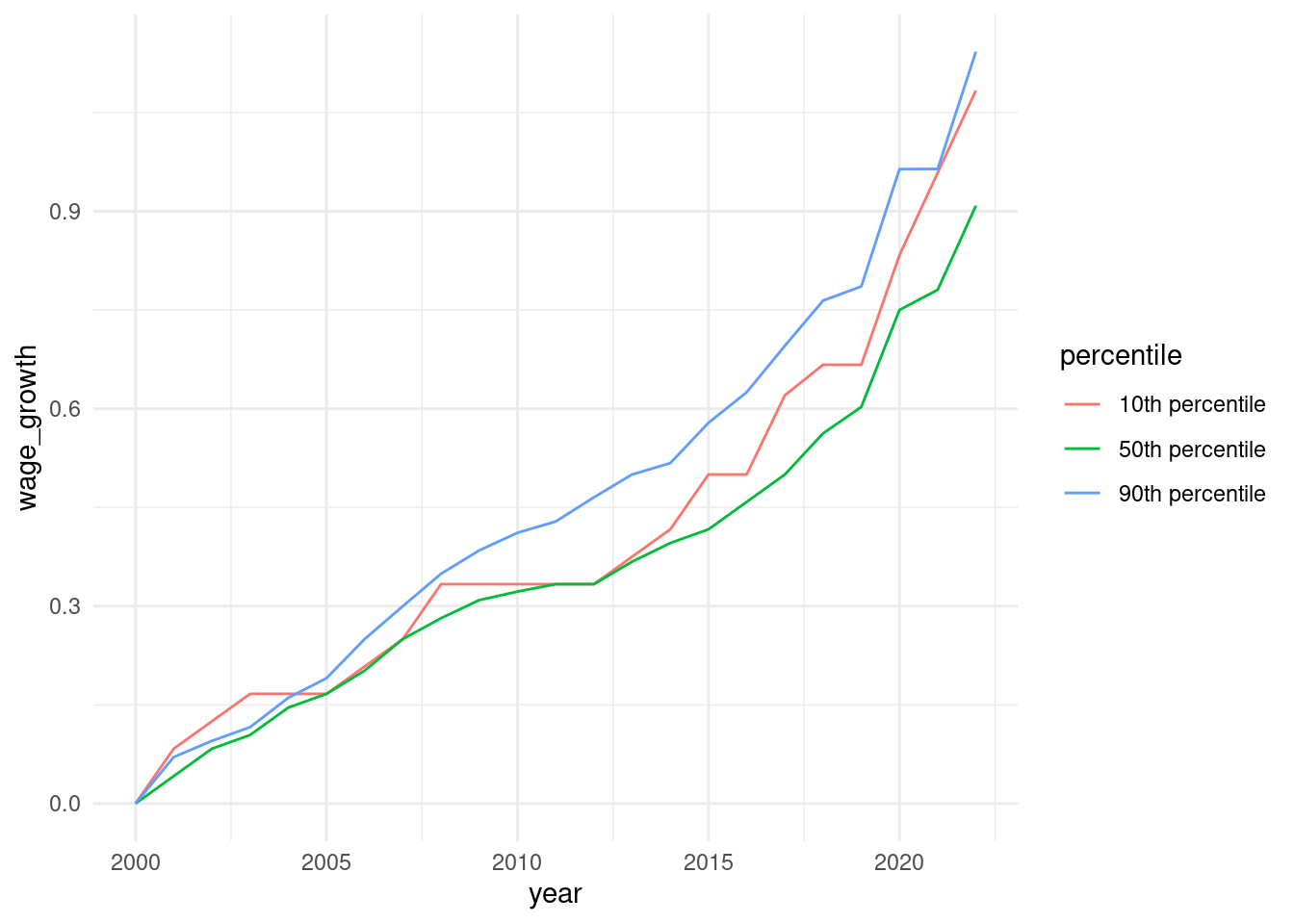

While long data like that is useful for additional analysis, if you need to see more of the data at once, like for a table, you might want to make the data wider. With pivot_wider() you can reshape the data so that it is long in years and wide in percentiles.

cps_data %>%
  reframe(
    percentile = p,
    value = weighted_quantile(wage, w = orgwgt, probs = p / 100),
    .by = year
  ) %>%
  pivot_wider(id_cols = year, names_from = percentile, values_from = value)

# A tibble: 44 × 4
    year  `10`  `50`  `90`
   <int> <dbl> <dbl> <dbl>
 1  1979  2.90  5     10.1
 2  1980  3.10  5.62  11.2
 3  1981  3.35  6.05  12.5
 4  1982  3.35  6.5   13.1
 5  1983  3.40  6.70  14  
 6  1984  3.5   7     15.0
 7  1985  3.5   7.47  15  
 8  1986  3.60  7.5   16  
 9  1987  3.75  8     16.8
10  1988  4     8.02  17.5
# ℹ 34 more rows

Of course, the column names are pretty ugly. You could add a “th” to the column names from the get-go.

cps_data %>%
  reframe(
    percentile = paste0(p, "th"),
    value = weighted_quantile(wage, w = orgwgt, probs = p / 100),
    .by = year
  ) %>%
  pivot_wider(id_cols = year, names_from = percentile, values_from = value)

# A tibble: 44 × 4
    year `10th` `50th` `90th`
   <int>  <dbl>  <dbl>  <dbl>
 1  1979   2.90   5      10.1
 2  1980   3.10   5.62   11.2
 3  1981   3.35   6.05   12.5
 4  1982   3.35   6.5    13.1
 5  1983   3.40   6.70   14  
 6  1984   3.5    7      15.0
 7  1985   3.5    7.47   15  
 8  1986   3.60   7.5    16  
 9  1987   3.75   8      16.8
10  1988   4      8.02   17.5
# ℹ 34 more rows

Or you could make the column names more data analysis friendly with a “p_” prefix.

cps_data %>%
  reframe(
    percentile = p,
    value = weighted_quantile(wage, w = orgwgt, probs = p / 100),
    .by = year
  ) %>%
  pivot_wider(
    id_cols = year,
    names_from = percentile,
    values_from = value,
    names_prefix = "p_"
  )

# A tibble: 44 × 4
    year  p_10  p_50  p_90
   <int> <dbl> <dbl> <dbl>
 1  1979  2.90  5     10.1
 2  1980  3.10  5.62  11.2
 3  1981  3.35  6.05  12.5
 4  1982  3.35  6.5   13.1
 5  1983  3.40  6.70  14  
 6  1984  3.5   7     15.0
 7  1985  3.5   7.47  15  
 8  1986  3.60  7.5   16  
 9  1987  3.75  8     16.8
10  1988  4     8.02  17.5
# ℹ 34 more rows

Extra credit

Consider the concise code

cps_data %>%
  reframe(
    name = p,
    value = weighted_quantile(wage, w = orgwgt, probs = p / 100),
    .by = year
  ) %>%
  pivot_wider(id_cols = year, names_prefix = "p_")

# A tibble: 44 × 4
    year  p_10  p_50  p_90
   <int> <dbl> <dbl> <dbl>
 1  1979  2.90  5     10.1
 2  1980  3.10  5.62  11.2
 3  1981  3.35  6.05  12.5
 4  1982  3.35  6.5   13.1
 5  1983  3.40  6.70  14  
 6  1984  3.5   7     15.0
 7  1985  3.5   7.47  15  
 8  1986  3.60  7.5   16  
 9  1987  3.75  8     16.8
10  1988  4     8.02  17.5
# ℹ 34 more rows

Why does it produce the same results as the longer code above?