library(tidyverse)
library(data.table) # setnames(), map DOL data dictionary to the raw data
library(lubridate) # data helper functions to recast messy data as date type
library(openxlsx2) # mapping data and setting formatting for excel wbForaging for Data in the Wild 2025
Welcome to the Foraging for Data in the Wild 2025 Landing page!
This training and code workflow was originally delivered as an EARN Talk on August 26th, 2025.
Missed this talk? See the recording here: Foraging for Data in the Wild.
Passcode: 4aging2025!
Unemployment Insurance Claims by State
1) Import libraries
2) Download raw data
UI IC & CC (NSA) comes for ETA 539, which can be found on the DOL ETA website.
Use the command-line utility function wget to trigger and direct the download of exportable online data. Wrap the statement in system() to direct execution to the terminal
NOTE: Some users encounter a 403 error with these commands. If this happens, manually download the ar539.csv file and place it in your working directory.
# "wget -N" omits download if data has not been updated "-P" sets the file destination"
system("wget -N https://oui.doleta.gov/unemploy/csv/ar539.csv  -P data/")
3) Wrangle data
Replace raw variable names using a user-defined data dictionary (download it here).
The data dictionary is a combination of the DOL ETA 539 Data Map (found on Data Downloads page) and the ETA 401 handook “Item by Item Instructions.”
# read in data dictionary
data_dictionary <- read.csv("data/eta539_var_names.csv")
4) Cleanse and manipulate data
Use data.table::setnames() to apply the data dictionary to the raw data. Recast date columns to be of Date class type (or data storage type). “Wild data” often stores dates as str (or string) class type, so use functions from the ?lubridate package to easily handle and manipulate date types.
# Cleanse raw data
raw_data <- read.csv("data/ar539.csv") |>
  # use $ operator to select column from data frame
  setnames(old = data_dictionary$dol_code, new = data_dictionary$dol_title) |>
  # format date as class 'Date'
  mutate(report_date = mdy(report_date),
         reflect_week_ending = mdy(reflect_week_ending))
5) Analyze
Use dplyr::mutate() to create new columns. Calculate non-seasonally adjusted initial claims as state UI initial claims + short-term compensation (or workshare) initial claims and non-seasonally adjusted continued claims as state UI continued claims + short-tern compensation (or workshare) continued claims.
# Initial claims (NSA)
initial_claims <- raw_data  |>
  # Initial Claims & Continued Claims, non seasonally adjusted (as seen here: https://oui.doleta.gov/unemploy/claims.asp)
  # UI IC is calculated from c3 (initial claims) & c7 (short time compensation workshare)
  mutate(nsa_initial_claims = state_ui_initial_claims + stc_workshare_equivalent_initial_claims) |>
  select(state, report_date, nsa_initial_claims) |>
  # filter out unstable reporting
  filter(report_date >= '1987-01-01') |>
  # transform into wide format - each state is own column
  #note: https://bookdown.org/Maxine/r4ds/pivoting.html
  pivot_wider(id_cols = report_date, names_from = state, values_from = nsa_initial_claims) |>
  # remove Puerto Rico and US Virgin Islands
  select(-PR, -VI) |>
  # replace state abbreviation with state name
  setnames(old = state.abb, new = state.name) |>
  # rename DC (not included in state* utility functions)
  rename(`District of Columbia` = DC) |>
  # sort data
  arrange(report_date)

# Continued claims (NSA)
continued_claims <- raw_data |>
  # Initial Claims & Continued Claims, non seasonally adjusted (as seen here: https://oui.doleta.gov/unemploy/claims.asp)
  # UI CC is calculated from c8 & c12
  mutate(nsa_continued_claims = state_ui_adjusted_continued_weeks_claimed + stc_workshare_equivalent_continued_weeks_claimed) |>
  select(state, reflect_week_ending, nsa_continued_claims) |>
  # filter out unstable reporting
  filter(reflect_week_ending >= '1987-01-01') |>
  # transform into wide format - each state is own column
  pivot_wider(id_cols = reflect_week_ending, names_from = state, values_from = nsa_continued_claims) |>
  # remove Puerto Rico & US Virgin Islands
  select(-PR, -VI) |>
  # replace state abbreviation with state name
  setnames(old = state.abb, new = state.name) |>
  # replace DC (not included in state.* utility data)
  rename(`District of Columbia` = DC) |>
  # sort data
  arrange(reflect_week_ending)
6) Export data
Use ?openxlsx2 to create excel workbooks, which support multiple tabs and backend formatting. This is a great way to generate replicable final products. Note that openxlsx2 uses the $ pipe operator to modify workbook objects created by openxlsx2::wb_workbook(). Create worksheets, add data, and use functions such as opnexlsx2::wb_set_col_widths() and openxlsx2::add_cell_style() to stylize the workbook.
# create WB object
wb <- wb_workbook()

# write UI state IC to WB object
#note: $ - pipe operator in openxlsx2
wb$
  # add new worksheet
  add_worksheet(sheet = "Initial claims")$
  # add data to worksheet
  add_data(x = initial_claims)$
  # set columm widths
  set_col_widths(cols = 2:ncol(initial_claims), widths = 15)$
  # format column headers
  add_cell_style(dims = wb_dims(rows = 1, cols = 2:ncol(initial_claims)),
                 wrap_text = TRUE, horizontal = "center", vertical = "center")$
  # repeat for continued claims
  add_worksheet(sheet = "Continued claims")$
  add_data(x = continued_claims)$
  set_col_widths(cols = 2:ncol(continued_claims), widths = 15)$
  add_cell_style(dims = wb_dims(rows = 1, cols = 2:ncol(continued_claims)),
                 wrap_text = TRUE, horizontal = "center", vertical = "center")$
  # save workbook to output folder
  save("output/state_ui.xlsx")
Using the QCEW to measure employment growth in data centers by state
Objectives
- Create data by iteratively calling a function.
- Bind/append data frames to create a large dataset.
- Read data from a .CSV directly from the web into R.
- Harmonize data types.
- Use joins to combine datasets.
- Filter using string detection.
- Reorder variables using
select(),arrange(), and/orrelocate()functions.- Use some tricks to create quarterly and monthly data types with
lubridate.- Measure employment changes for NAICS industry 518.
- Bonus: quick visualization with ggplot2!
Question. How has “data center” employment (NAICS 518) grown since late 2022, and in which states has it grown the most?
To answer these questions, we’ll fetch 2022–2024 quarterly data for NAICS 518: Computing infrastructure providers, data processing, web hosting, and related services.
** Disclaimer**: I’m not sure if this is the most appropriate NAICS code, but it makes for a good exercise! Depending on your research question, you may want to refine how you select industry codes (e.g., include selected sub‑industries or complementary sectors.).
1) Load libraries
library(tidyverse)
library(lubridate)
2) BLS functions for loading QCEW data
The BLS conveniently provides a script and three functions for R users to load QCEW data directly into R! Below are two helpers adapted for this module. They construct an API URL and return a data frame for the requested year/quarter/industry or area.
These resources can be downloaded from this page: https://www.bls.gov/cew/additional-resources/open-data/sample-code.htm#RSCRIPT
# This function loads all industries for one geographical area
qcewGetAreaData <- function(year, qtr, area) {
  url <- "http://data.bls.gov/cew/data/api/YEAR/QTR/area/AREA.csv"
  url <- sub("YEAR", year, url, ignore.case=FALSE)
  url <- sub("QTR", tolower(qtr), url, ignore.case=FALSE)
  url <- sub("AREA", toupper(area), url, ignore.case=FALSE)
  read.csv(url, header = TRUE, sep = ",", quote="\"", dec=".", na.strings=" ", skip=0)
}

# This function loads one industry for all geographical areas
qcewGetIndustryData <- function (year, qtr, industry) {
    url <- "http://data.bls.gov/cew/data/api/YEAR/QTR/industry/INDUSTRY.csv"
    url <- sub("YEAR", year, url, ignore.case=FALSE)
    url <- sub("QTR", tolower(qtr), url, ignore.case=FALSE)
    url <- sub("INDUSTRY", industry, url, ignore.case=FALSE)
    read.csv(url, header = TRUE, sep = ",", quote="\"", dec=".", na.strings=" ", skip=0)
}

# Quick examples (not evaluated by default)
# In ex. 1, we call the qcewGetAreaData() function, passing parameters for year, quarter, and areafips/geography i.e. year = 2015, quarter = 1, areafips = 26000 or Michigan.
# We then assign the data called to a variable called MichiganData!

#  MichiganData <- qcewGetAreaData("2015", "1", "26000")
#  Construction <- qcewGetIndustryData("2015", "1", "1012")
3) QCEW data pull
Since the example functions load only one quarter at a time, we’ll want to make some modifications. Instead of calling the function 12 times by hand, we’ll build a grid of parameters and map across it.
# Set our parameters
years <- 2022:2024
quarters <- 1:4
industries <- c('518')

# create 12 combinations (3 years × 4 quarters × 1 industry) to pass through pmap()
combos <- tidyr::crossing(year = years, qtr = quarters, industry = industries)

# Takes the combinations, runs qcewGetIndustryData() once for each
# returns a list of "small" dataframes, which we combine into a large one called QCEW raw

qcew_raw <- pmap(combos, function(year, qtr, industry){
  qcewGetIndustryData(year, qtr, industry)
  }) |>
  # Combines all dataframes by appending/binding "rows"
  bind_rows()

# Explores our data
glimpse(qcew_raw)
Rows: 29,108
Columns: 42
$ area_fips <chr> "01000", "01000", "01001", "01003", "0…
$ own_code <int> 2, 5, 5, 5, 5, 5, 5, 5, 5, 5, 5, 5, 5,…
$ industry_code <int> 518, 518, 518, 518, 518, 518, 518, 518…
$ agglvl_code <int> 55, 55, 75, 75, 75, 75, 75, 75, 75, 75…
$ size_code <int> 0, 0, 0, 0, 0, 0, 0, 0, 0, 0, 0, 0, 0,…
$ year <int> 2022, 2022, 2022, 2022, 2022, 2022, 20…
$ qtr <int> 1, 1, 1, 1, 1, 1, 1, 1, 1, 1, 1, 1, 1,…
$ disclosure_code <chr> "", "", "N", "", "N", "", "N", "N", "N…
$ qtrly_estabs <int> 1, 1019, 2, 31, 1, 4, 2, 1, 1, 0, 1, 6…
$ month1_emplvl <int> 13, 2421, 0, 72, 0, 7, 0, 0, 0, 0, 0, …
$ month2_emplvl <int> 13, 2511, 0, 73, 0, 7, 0, 0, 0, 0, 0, …
$ month3_emplvl <int> 13, 2523, 0, 79, 0, 7, 0, 0, 0, 0, 0, …
$ total_qtrly_wages <dbl> 249734, 60137580, 0, 1271327, 0, 67735…
$ taxable_qtrly_wages <dbl> 0, 20180327, 0, 574492, 0, 47119, 0, 0…
$ qtrly_contributions <int> 0, 322219, 0, 8174, 0, 2132, 0, 0, 0, …
$ avg_wkly_wage <int> 1478, 1862, 0, 1310, 0, 744, 0, 0, 0, …
$ lq_disclosure_code <chr> "", "", "N", "", "N", "", "N", "N", "N…
$ lq_qtrly_estabs <dbl> 4.05, 1.81, 0.51, 1.06, 0.29, 0.39, 0.…
$ lq_month1_emplvl <dbl> 1.07, 0.40, 0.00, 0.31, 0.00, 0.05, 0.…
$ lq_month2_emplvl <dbl> 1.06, 0.42, 0.00, 0.31, 0.00, 0.05, 0.…
$ lq_month3_emplvl <dbl> 1.05, 0.42, 0.00, 0.33, 0.00, 0.05, 0.…
$ lq_total_qtrly_wages <dbl> 1.29, 0.30, 0.00, 0.21, 0.00, 0.02, 0.…
$ lq_taxable_qtrly_wages <dbl> 0.00, 0.33, 0.00, 0.25, 0.00, 0.04, 0.…
$ lq_qtrly_contributions <dbl> 0.00, 0.40, 0.00, 0.27, 0.00, 0.15, 0.…
$ lq_avg_wkly_wage <dbl> 1.21, 0.73, 0.00, 0.65, 0.00, 0.36, 0.…
$ oty_disclosure_code <chr> "N", "", "N", "", "N", "", "N", "N", "…
$ oty_qtrly_estabs_chg <int> 0, 318, 0, 10, 1, 0, 1, -1, 1, 0, 0, 1…
$ oty_qtrly_estabs_pct_chg <dbl> 0.0, 45.4, 0.0, 47.6, 100.0, 0.0, 100.…
$ oty_month1_emplvl_chg <int> 0, 149, 0, 0, 0, 3, 0, 0, 0, 0, 0, -1,…
$ oty_month1_emplvl_pct_chg <dbl> 0.0, 6.6, 0.0, 0.0, 0.0, 75.0, 0.0, 0.…
$ oty_month2_emplvl_chg <int> 0, 216, 0, 0, 0, 2, 0, 0, 0, 0, 0, -1,…
$ oty_month2_emplvl_pct_chg <dbl> 0.0, 9.4, 0.0, 0.0, 0.0, 40.0, 0.0, 0.…
$ oty_month3_emplvl_chg <int> 0, 201, 0, 3, 0, 2, 0, 0, 0, 0, 0, -1,…
$ oty_month3_emplvl_pct_chg <dbl> 0.0, 8.7, 0.0, 3.9, 0.0, 40.0, 0.0, 0.…
$ oty_total_qtrly_wages_chg <dbl> 0, 13354348, 0, 210886, 0, 5327, 0, 0,…
$ oty_total_qtrly_wages_pct_chg <dbl> 0.0, 28.5, 0.0, 19.9, 0.0, 8.5, 0.0, 0…
$ oty_taxable_qtrly_wages_chg <int> 0, 2694560, 0, 39716, 0, 12909, 0, 0, …
$ oty_taxable_qtrly_wages_pct_chg <dbl> 0.0, 15.4, 0.0, 7.4, 0.0, 37.7, 0.0, 0…
$ oty_qtrly_contributions_chg <int> 0, -46111, 0, -4990, 0, 371, 0, 0, 0, …
$ oty_qtrly_contributions_pct_chg <dbl> 0.0, -12.5, 0.0, -37.9, 0.0, 21.1, 0.0…
$ oty_avg_wkly_wage_chg <int> 0, 295, 0, 203, 0, -285, 0, 0, 0, 0, 0…
$ oty_avg_wkly_wage_pct_chg <dbl> 0.0, 18.8, 0.0, 18.3, 0.0, -27.7, 0.0,…4) Add readable labels (industry & area titles)
Our dataframe is loaded! But it’s not very legible. For starters, some geographic and industry titles would help.
The BLS provides a codebook for parsing our data https://www.bls.gov/cew/about-data/downloadable-file-layouts/quarterly/naics-based-quarterly-layout.htm. We’ll load these directly into R.
** disclaimer ** depending on your IT’s security settings, you may not be able to directly download these links into R. If you encounter this issue (like I did), you can navigate directly to the .htm links below, download the .CSV files, and place them in your working directory.
Industry titles downloaded from https://www.bls.gov/cew/classifications/industry/industry-titles.htm
Area titles downloaded from https://www.bls.gov/cew/classifications/areas/qcew-area-titles.htm
# link to csv files on the BLS QCEW site
ind_title_url <- 'https://www.bls.gov/cew/classifications/industry/industry-titles.csv'
area_title_url <- 'https://www.bls.gov/cew/classifications/areas/area-titles-csv.csv'

# # Read csv files directly into R from the QCEW page
# ind_titles  <- read_csv(ind_title_url)
# area_titles <- read_csv(area_title_url)

ind_titles <- read_csv('data/industry_titles.csv')
area_titles <- read_csv('data/area-titles-csv.csv')
4a) First attempt at joining labels
We’ll first attempt a natural left_join() on industry_code. A left join keeps all rows from our main dataset (qcew, the “x” table) and adds matches from ind_titles (the “y” table). By default, it matches on any identically named columns (a “natural join”), but we could also set the key explicitly using the by = argument.
See Section 19.4 How do joins work? from R for Data Science (2e) for some great visualizations.
# Can you spot the difference?
glimpse(qcew_raw$industry_code)   # likely <int> / <dbl>
int [1:29108] 518 518 518 518 518 518 518 518 518 518 ...glimpse(ind_titles$industry_code) # likely <chr> chr [1:2678] "10" "101" "1011" "1012" "1013" "102" "1021" "1022" "1023" ...# What happens?
qcew_raw |>
dplyr::left_join(ind_titles)Joining with `by = join_by(industry_code)`Error in `dplyr::left_join()`:
! Can't join `x$industry_code` with `y$industry_code` due to
incompatible types.
ℹ `x$industry_code` is a <integer>.
ℹ `y$industry_code` is a <character>.4b) Harmonizing data types to join
Maldito! We have an issue. Despite matching variable names, industry_code in datasets “x” and “y” are different datatypes. in “x”, it’s an integer, a numeric type. in “y” it’s a character. In order to merge we need our datatypes to be the same.
Fortunately, is an easy fix. We can convert one of two columns to match data types. Which should we convert? Well, it’s easier to go from character to numeric here. A quirk of R is that numerics don’t have leading zeros, but strings can. You wouldn’t write 100 as 0100, or 00100, right? Right??
Since NAICS 3‑digit codes like 518 don’t have leading zeros, converting ind_titles$industry_code to numeric is safe here. (General tip: if codes are required to have leading zeros, keep them as character in both tables.)
# Make the join keys the same type
ind_titles <- ind_titles |>
  mutate(industry_code = as.numeric(industry_code))
Warning: There was 1 warning in `mutate()`.
ℹ In argument: `industry_code = as.numeric(industry_code)`.
Caused by warning:
! NAs introduced by coercion# Now the join works:
qcew_ind_clean <- qcew_raw |>
# natural join on identical names
left_join(ind_titles) Joining with `by = join_by(industry_code)`# We could also be explicit about which variable to join by
# qcew_ind_clean <- qcew_raw |>
# left_join(ind_titles, by = 'industry_code')
# If our variable names differ, we could map them using
# left_join(ind_titles, by = c("industry_code" = "ind_code"))4c) Cleaning continued
Now join titles and keep only variables we need. We also want limit to private‑sector, statewide data only. We know from the QCEW codebook that: own_code == 5 and agglvl_code == 55.
See this codebook for more detail: QCEW Field Layouts for NAICS-Based, Quarterly CSV Files
# (If needed) ensure area_fips types match before joining area_titles
# area_titles <- area_titles |> mutate(area_fips = as.character(area_fips))

qcew_clean <- qcew_ind_clean |>
  left_join(area_titles) |>
  # Too many variables we don't need, let's restrict and re-order using select
  select(
    year, qtr, area_fips, area_title, industry_code,
    industry_title, own_code, agglvl_code, month1_emplvl, month2_emplvl,
    month3_emplvl) |>

  # Now, why are seeing two rows for each state? Again, per the codebook, QCEW contains data for public and private sector industries
  # We can filter for private sector data using own_code == 5
  filter(own_code == 5) |>
  filter(agglvl_code == 55)
Joining with `by = join_by(area_fips)`# Tip: An alternative way to filter for statewide data. If you don’t have a variable like agglvl_code, you can use string detection to filter statewide rows. We prefer to use code‑book filters when available.
# filter(str_detect(area_title, " -- Statewide")) 5) Quarterly dates & averages
Create a quarterly average employment measure and a proper quarterly date using lubridate’s yq().
qcew_qtr <- qcew_clean |>
  mutate(
    qtr_avg_emp = (month1_emplvl + month2_emplvl + month3_emplvl) / 3,
    qdate       = yq(paste(year, qtr, sep = " Q"))
  )
6) Reshape to create state‑by‑column tables
Now that we have quarterly data, we’ll use pivot_wider() to create a table of quarterly data that is long by date.
state_qtr_table <- qcew_qtr |>
  mutate(state = str_replace(area_title, " -- Statewide", "")) |>
  select(qdate, state, qtr_avg_emp) |>
  pivot_wider(id_cols = qdate, names_from = state, values_from = qtr_avg_emp)

state_qtr_table
# A tibble: 12 × 54
qdate Alabama Alaska Arizona Arkansas California Colorado Connecticut
<date> <dbl> <dbl> <dbl> <dbl> <dbl> <dbl> <dbl>
1 2022-01-01 2485 96.3 12099. 4383. 66262. 16167. 3649.
2 2022-04-01 2772. 108 12538. 4546. 71640. 16592 3759.
3 2022-07-01 3060. 112. 12322 4705. 72875 16611. 3883.
4 2022-10-01 3143 97.3 12230 4746. 74211 16504 3795.
5 2023-01-01 3563. 117. 12441 4786. 84623 16157 3795
6 2023-04-01 3699. 132. 12235. 4589 83776. 15891. 3778
7 2023-07-01 3872 131. 11652. 4521. 83244. 15563 3750.
8 2023-10-01 3875 121 11905. 4494. 81299 15325. 3755.
9 2024-01-01 3738 108. 11401 4328 79753. 15234. 4081.
10 2024-04-01 3812. 110. 11726. 4184. 79390. 15184 4314.
11 2024-07-01 3929 130. 11374. 4170. 79600 15082. 4371
12 2024-10-01 3941 119. 11179. 4136. 78681. 14996. 4311.
# ℹ 46 more variables: Delaware <dbl>,
# `District of Columbia, not unknown` <dbl>, Florida <dbl>, Georgia <dbl>,
# Hawaii <dbl>, Idaho <dbl>, Illinois <dbl>, Indiana <dbl>, Iowa <dbl>,
# Kansas <dbl>, Kentucky <dbl>, Louisiana <dbl>, Maine <dbl>, Maryland <dbl>,
# Massachusetts <dbl>, Michigan <dbl>, Minnesota <dbl>, Mississippi <dbl>,
# Missouri <dbl>, Montana <dbl>, Nebraska <dbl>, Nevada <dbl>,
# `New Hampshire` <dbl>, `New Jersey` <dbl>, `New Mexico` <dbl>, …7) Monthly data from QCEW
The QCEW provides monthly employment levels in each quarter! With a few tweaks to our data frame, we can produce a monthly series, giving us a more granular look at how data center employment has grown since 2022. Each QCEW quarter reports employment for its three months. We can unpivot those columns to build a monthly time series.
qcew_monthly <- qcew_clean |>
  pivot_longer(
    cols = starts_with("month"),
    names_to = "month_in_qtr",
    names_pattern = "month(\\d+)_emplvl",
    values_to = "emplvl"
  ) |>
  mutate(
    month_in_qtr = as.integer(month_in_qtr),
    month        = (qtr - 1) * 3 + month_in_qtr,
    date         = make_date(year, month, 1),
  ) |>
  select(area_title, area_fips, industry_code, year, qtr, date, emplvl) |>
  arrange(area_title, year, qtr, date) |>
  # let's clean up our state names!
  mutate(state = str_replace(area_title, " -- Statewide", ""))

head(qcew_monthly)
# A tibble: 6 × 8
area_title area_fips industry_code year qtr date emplvl state
<chr> <chr> <dbl> <int> <int> <date> <int> <chr>
1 Alabama -- Statew… 01000 518 2022 1 2022-01-01 2421 Alab…
2 Alabama -- Statew… 01000 518 2022 1 2022-02-01 2511 Alab…
3 Alabama -- Statew… 01000 518 2022 1 2022-03-01 2523 Alab…
4 Alabama -- Statew… 01000 518 2022 2 2022-04-01 2722 Alab…
5 Alabama -- Statew… 01000 518 2022 2 2022-05-01 2795 Alab…
6 Alabama -- Statew… 01000 518 2022 2 2022-06-01 2798 Alab…8) Measure employment growth since late 2022
For a simple comparison, compute percentage change from November 2022 to the latest available month for each state. (If a state is missing November specifically, we’ll use the first available month on or after 2022‑11‑01.)
state_growth <- qcew_monthly |>
  summarize(
    start_emplvl = first(emplvl),
    end_emplvl   = last(emplvl),
    start_date   = first(date),
    end_date     = last(date),
    .by=state) |>
  mutate(
    emp_change = (end_emplvl - start_emplvl),
    pct_change = (end_emplvl / start_emplvl - 1) * 100) |>
  # arrange data in descending order by pct_change
  arrange(desc(pct_change))

state_growth |> slice_head(n = 10)
# A tibble: 10 × 7
state start_emplvl end_emplvl start_date end_date emp_change pct_change
<chr> <int> <int> <date> <date> <int> <dbl>
1 Alabama 2421 3929 2022-01-01 2024-12-01 1508 62.3
2 Idaho 903 1296 2022-01-01 2024-12-01 393 43.5
3 South Da… 293 405 2022-01-01 2024-12-01 112 38.2
4 Alaska 89 120 2022-01-01 2024-12-01 31 34.8
5 Wyoming 163 217 2022-01-01 2024-12-01 54 33.1
6 New Jers… 12474 16072 2022-01-01 2024-12-01 3598 28.8
7 Maryland 4377 5631 2022-01-01 2024-12-01 1254 28.6
8 Rhode Is… 625 787 2022-01-01 2024-12-01 162 25.9
9 New Hamp… 1465 1822 2022-01-01 2024-12-01 357 24.4
10 West Vir… 1182 1439 2022-01-01 2024-12-01 257 21.79) Bonus: Making a quick visualization
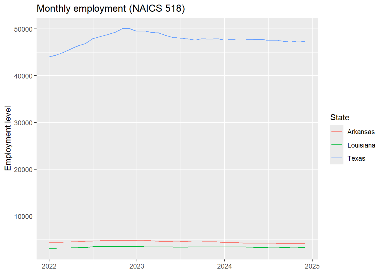
Lets plot a few states using ggplot2
P.S. check out viz_workshop.qmd for some more ggplot examples!
sel_state_data <- qcew_monthly |>
  filter(state %in% c('Texas', 'Arkansas', 'Louisiana'))

ggplot(data = sel_state_data, aes(x=date, y=emplvl, color=state)) +
  geom_line() +
  labs(
    title = "Monthly employment (NAICS 518)",
    x = NULL, y = "Employment level",
    color = "State"
) 
10) Notes on reproducibility
Pro-tips: - This module reads files directly from bls.gov; those URLs occasionally change. If a link breaks, visit the QCEW classifications pages to refresh the URLs. - Consult QCEW layout/codebook to confirm variable meanings & aggregation levels for your projects.
Happy coding!🕺